LBO model tutorial with free Excel

The acquisition of another company using a significant amount of borrowed money (bonds or loans) to meet the cost of an acquisition is named a Leveraged Buyout Analysis. It is used to determine an implied valuation range for a given target in a potential LBO sale based on achieving acceptable returns.

Step by step LBO Valuation tutorial

In these coming four steps, you will be able to perform your own LBO Analysis. This LBO model is simplified in order to teach you the basics of a LBO valuation.

Start by downloading this LBO model for Excel (it is 100% free and takes less than 1 minute to download). All required inputs will be described in detail below.

USE CODE: BVAL100 for 100% discount.

Expand each section to follow the (free!) LBO-model tutorial. Now lets do some modeling!

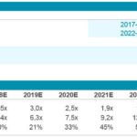
Sneak peek of the LBO model (click to enlarge screenshots)

You need to activate “iterations” in Excel for this LBO model to work properly. It can be switched on under Excel options / formulas / then check the box “Enable iterative calculations”. See picture here for help (if needed).

Step 1 - Enter Deal Value
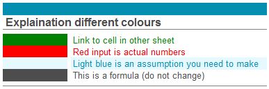
Before we can start the modeling, it is important that you understand the coloring of the LBO Excel sheet. Please see description below. Always be consistent with colouring when you model, since it will help you in the long run.

Explaination Excel colours

Deal inputs

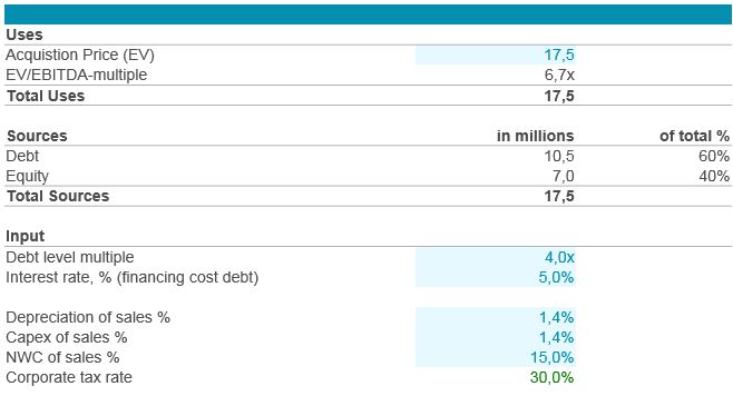
Okey, now let us get into the action. We will start with the input in the below screenshot.

Deal inputs

Steps

  1. USES: Enter the acquisition price, in this example we were offered to buy this company for 17.5 million which implied a 6.7x EV/EBITDA-multiple.
  2. INPUT: What leverage will your acquisition have? We have chosen to borrow 4x times EBITDA, which is a “normal” leverage. In our example, this implies 60% of total uses, implying that we need to add 7 million equity in order to fund this LBO.
  3. Enter the interest rate at which you can borrow money at. In this example we assume a 5% interest rate.
  4. Make an assumption of depreciation in % of net sales to be used in the forecast period. Look at historical ratios for guidance.
  5. Input CAPEX in % to sales. If you do not know, look at historical values found in the annual report
  6. Enter NWC (Net working capital) in percentage of sales. Look at historical values if you do not know
Step 2 - Enter historical financials

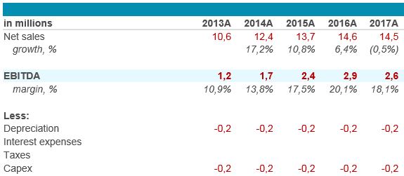
In this step you need to enter historical financials of Net sales, EBITDA, Depreciation and CAPEX. All these entries are red in current Excel to make it easier for you *love*.

Deal inputs

Deal inputs historical trading

Steps

  1. Enter net sales, EBITDA, depreciation and CAPEX.
Step 3 - Forecast period

In this step we will try to make assumptions of growth and profitability for the forecast period. We are also adding a scenario analysis (Base case, Best case and Low case).
Forecast and case selector

Steps

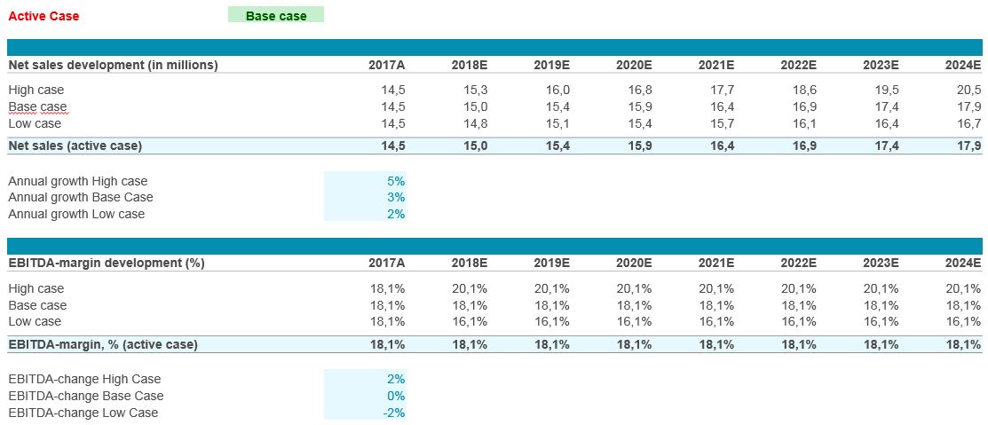
  1. The scenario which is active is determined by the drop down in the sheet LBO model, cell D2. This cell determines what should be used in the LBO model and affects line 11 and line 24 in the Case selector sheet.
  2. Go to the Case selector sheet in the Excel spread sheet
  3. Make assumptions of annual sales growth in the Base case, High and in the Low case (Column D and line 13-15).
  4. Enter the assumed EBITDA margin for each year. You can either make own predictions for each year, or use same margins throughout the forecast period. Elaborate with these numbers to adjust for your business. We have tried to keep it simple. Our assumptions are made in column D26-28 (+-2%).

Output

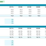
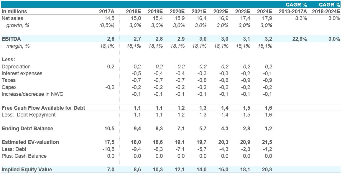
Now, you have almost made all needed assumptions. See picture below for a beautiful output (adjust as needed):

Result of LBO

Step 4 - Understanding the results and output

Almost done… But first we need to make the exit assumptions. We use the same EBITDA multiple as when we bought it 6.7x times EBITDA (see input below). No action needed unless you want other assumptions.
Exit assumptions

Output

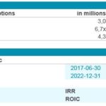
The LBO valuation is done. Below are the results for our example company:

Credit statistics

Understanding the results

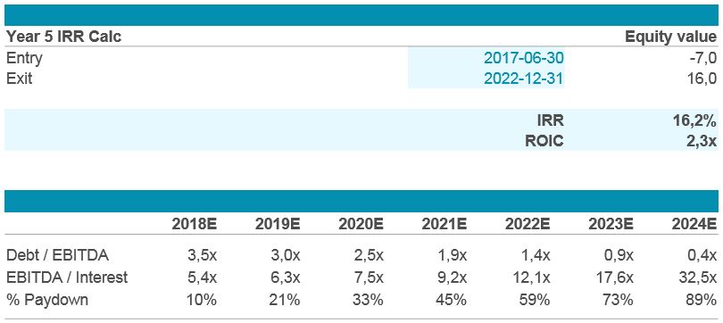
  1. We paid 7 million in equity on the entry date (2017-06-30). Change Date in cell C32.
  2. We will get 16 million cash when we sell the company in five years (2022-12-31). During these five years we have paid interest on the debt and amortized more than half of the debt in Base case.
  3. This implies an internal rate of return (IRR) of 16.2%
  4. We have doubled our initial equity stake 2.3x (ROIC) times during this period
  5. Some financial ratios are also supplied in the output (pretty straight forward / easy!)
It would mean the world to me if you could help me with a 5-star rating here and possibly also some nice comments, if you have completed this tutorial successfully.

This will encourage me to continue to develop the best Excel models and will take very little of your time…

Any questions??

Business valuation proI will do my best to help you quick

I will gladly help you with any question you might have. Either comment below the relevant content or send me an email or use my contact form which can be found here.

Specialities: Business valuations, Excel models, Business development, Investment Banking, Buyouts, Divestments, Share issues, IPOs, Management Buyouts, Leveraged Buyouts.

Have a great day! (thanks for sharing my website which helps my content available to more users)
 

9 thoughts on “LBO model tutorial with free Excel

  1. Where do I input how much debt the company takes in in order to finance the LBO?

    How do I calcuate that part?

    Thank you in advance

  2. Thank you very much for this comprehensively-explained LBO Model. However, this model assumes the target has no existing debt. Do you have such LBO models with existing debt of target? Many Many Thanks

  3. Step 4 – Understanding the Results section has a typo. It says the IRR is 17%, but really it is 19% (as the picture above the comment, and the model itself, both correctly reflect).

Leave a Reply

Your email address will not be published. Required fields are marked *

15 − seven =